39 excel pivot table conditional formatting row labels

How to Remove Blanks in a Pivot Table in Excel (6 Ways) To apply conditional formatting to remove blanks in a pivot table: Click in the pivot table. Press Ctrl + A to select the cells. Click the Home tab in the Ribbon and click Conditional Formatting. A drop-down menu appears. Select New Rule. A dialog box appears. In the dialog box, click Format only cells that contain. Excel Conditional Formatting in Pivot Table - EDUCBA Click on any cell in the pivot table > Go to the HOME tab > Click on Conditional Formatting option under Styles option > Click on Manage Rules option. It will open a Rules Manager dialog box. Click on the Edit Rule tab, as shown in the below screenshot. It will open the Editing Rule formatting window. Refer to the below screenshot.

101 Advanced Pivot Table Tips And Tricks ... - How To Excel Apr 25, 2022 · Without a table your range reference will look something like above. In this example, if we were to add data past Row 51 or Column I our pivot table would not include it in the results. To create and name your table. Select your data. Go to the Insert tab and press the Table button in the Tables section, or use the keyboard shortcut Ctrl + T.

Excel pivot table conditional formatting row labels

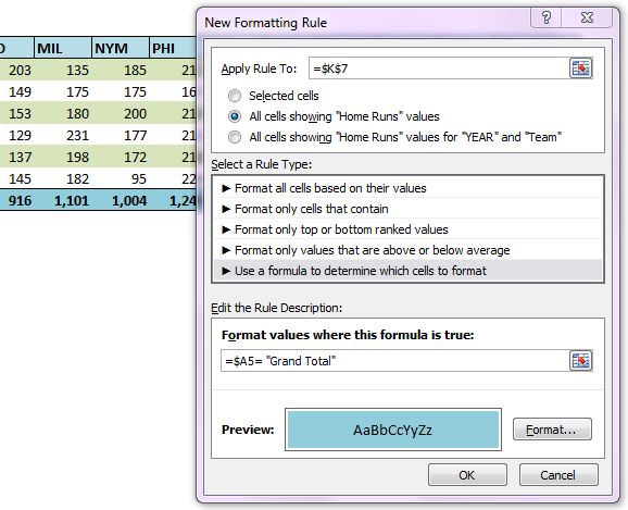
Conditional Format Pivot Table Row - Chandoo.org Excel Ninja Apr 3, 2013 #2 Select the entire row, and when you apply the conditional format, make the column reference absolute. So, say we want the entire row 2 to be formatted if cell in col B = 5. formula would be: =$B2=5 Conditional formatting for Pivot Tables in Excel 2016 ... The format I used was to select Conditional Formatting > Top 10 Items > set it to 1 item and select the default format. This format can be copied from one range to the next if desired or built up for each range individually. To copy the format, select one or more cells with that format and click Copy. How to Highlight A row based on Cell Value In Pivot Table Basically, pivot tables were used to summarize a huge data. Meanwhile, conditional formatting is used to highlight a value with a logical connection. But, Can a particular cell value gets highlighted using conditional formatting?. This article provides the user with inputs required to highlight a row based on cell value in pivot table.

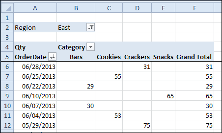
Excel pivot table conditional formatting row labels. Apply Conditional Formatting | Excel Pivot Table Tutorial Go to Home Tab → Styles → Conditional Formatting → New Rule. From rule to, select the third option. And, from "select a rule" type select "Format only top or bottom" ranked values. In edit rule description, enter 1 in the input box and from the drop-down menu select "each Column Group". Apply formatting you want. Click OK. Format Pivot Table Labels Based on Date Range - Excel ... Select all the dates in the Row Labels that you want to format. On the Ribbon, click the Home tab, and then in the Styles group, click Conditional Formatting. In the list of conditional formatting options, click Highlight Cells Rules, and then click A Date Occurring. Pivot Table Conditional Formatting Weekend Data Highlight Follow these steps to apply the weekend highlighting in the pivot table: Select all cells where conditional formatting should be applied, cells B5 to B20 in this example. On the Excel Ribbon, click the Home tab. Click Conditional Formatting, and in the drop down menu, click New Rule. The New Formatting Rule dialog box opens. Pivot Table Conditional Formatting with VBA - Peltier Tech It seems to occur because in 2007, conditional format is applied to a field, whereas in 2003, it's applied to a range. Without resorting to macros, it's possible to quickly reapply the conditional format in 2007 by following these steps: - Set the conditional format to range covering more than the pivot table (e.g. on cell above).

Formatting - Pivot Table Select all the dates in the Row Labels that you want to format. On the Ribbon, click the Home tab, and then in the Styles group, click Conditional Formatting. In the list of conditional formatting options, click Highlight Cells Rules, and then click A Date Occurring. In the date range drop-down, select Next Month, and then click the arrow to ... conditional formatting per row on pivot - Microsoft Tech ... conditional formatting per row on pivot. Hi, I would like to format each row of a pivot table separately (as in the picture shown below), but I cannot paste the formatting. I've got many rows, and they could change (just like the columns) How to preserve formatting after refreshing pivot table? In the PivotTable Options dialog box, click Layout & Format tab, and then check Preserve cell formatting on update item under the Format section, see screenshot: 4. And then click OK to close this dialog, and now, when you format your pivot table and refresh it, the formatting will not be disappeared any more. Conditionally Format Values Area Based on Row Labels (LONG) Conditionally Format Values Area Based on Row Labels (LONG) The Row Labels area is one column of job role titles (e.g., Project Manager, System Architect etc.). The Column Labels area includes 6 columns, each of which corresponds to 1 of 6 columns in the source data.

› documents › excelHow to make row labels on same line in pivot table? Please do as follows: 1. Click any cell in your pivot table, and the PivotTable Tools tab will be displayed. 2. Under the PivotTable Tools tab, click Design > Report Layout > Show in Tabular Form, see screenshot: 3. And now, the row labels in the pivot table have been placed side by side at once, see screenshot: answers.microsoft.com › en-us › msofficeConditional formatting in pivot tables using rows - Microsoft ... Oct 07, 2013 · Conditional formatting in pivot tables using rows. I am hoping someone can tell me how I can conditionally format pivot table data cells based on the value of the row categorization. I have a simple pivot that splits the data across rows based on ranges, e.g. 600-650, 550-600 etc. I want to tell Excel to use a specific fill color for any cell on the same row as a specific row label, so for example if the row label value is "600-650" the data cells on the table will be filled in yellow etc. How to Apply Conditional Formatting to Pivot Tables ... Dec 13, 2018 · Bottom Line: Learn how to apply conditional formatting to pivot tables so that the formats are dynamically reapplied as the pivot table is changed, filtered, or updated. Skill Level: Intermediate Download the Excel File. Here's the file that I use in the video. You can use it to practice adding, deleting, and changing conditional formatting on a variety of pivot table … Conditional formatting rows in a pivot table based on one ... What you need to do is accept the formula the way you type it, close the conditional formatting rules manager and then reopen it. Remove the $ from the row numbers that excel added into your formula but leave it on the column number like so =$I3=992, or whatever your first row is.

How to Apply Data Bars in Pivot Table - MS Excel | Excel In Excel

Conditional Formatting PivotTables - My Online Training Hub Here's a step by step how to: 1. Select any cell in the values area of your PivotTable. 2. On the Home tab of the Ribbon select Conditional Formatting > Top/Bottom Rules > Top 10 Items: 3. Set the value to 1 and choose your format: 4. You will now have an icon beside the cell that you have applied the formatting to.

Sorting a Pivot Table - Free Microsoft Excel Tutorials

excel - How can I make my conditional formatting macro ... I have a pivot table where the rows contain some categories and the columns contain dates in ascending order and the values in the table are $ amounts. I am running a macro which puts the same 'amount' field in the 'values' box again and then I use 'show as difference from' to see the changes in the amounts b/w different dates.

How to Create a MS Excel Pivot Table – An Introduction | SIMPLE TAX INDIA

Conditional formatting formula in a table - Exceljet This is because structured references are not recognized inside a conditional formatting rule. The workaround is to use regular references. In this case, I need to use: F5 equals A, with column F locked. = $F5 = "A" This allows the formula to highlight an entire row. Now I'll use this formula to create the conditional formatting rule.

How To Find And Remove Duplicates In A Pivot Table - MS Excel | Excel In Excel

Excel Pivot Tables to Extract Data - My Online Training Hub Aug 02, 2013 · When I insert my Pivot Table Excel will use the Table name as the source range. ... is actually a row label and it’s expected that the row labels will have a name, not be blank. ... Creating an Excel PivotTable Profit and Loss Statement means you can use Slicers and Conditional Formatting and have the P&L automatically update.

Design your Pivot Table in Excel | Excel in Excel

Excel Pivot Table - Format Numbers in Rows To format rows or columns in a PT, hover the mouse at the top of the column or beginning of the row until a black arrow appears, click to highlight the row/column and format as usual. For Display labels from next field in same column, uncheck this, follow above procedure, then recheck. Paula Scharf.

Format Pivot Table Labels Based on Date Range – Excel Pivot Tables

Conditional formatting of pivot table by row label Conditional formatting of pivot table by row label. I would like to format my pivot table so that the alternative row labels are highlighted when the table is in tabular format. Here is an example of the desired formatting: New Bitmap Image.jpg. Thanks in advance!

Re-Apply Pivot Table Conditional Formatting - yoursumbuddy

› excel-charting-and-pivotsConditional Formatting on Pivot Table row labels As per my knowledge, in this case it does not matter what is the source of pivot as after getting the data in pivot, it's the pivot where the conditional formatting need to be applied, please upload a sample. thanks. Regards, DILIPandey DILIPandey +91 9810929744 dilipandey@gmail.com Register To Reply

Share :